SIFT

Useful Materials

1. Distinctive Image Features from Scale-Invariant Keypoints^[1] by David G. Lowe.

2. SIFT(Scale-Invariant Feature Transform)^[2] on Towards Data Science.

3. The SIFT (Scale Invariant Feature Transform) Detector and Descriptor^[3].

Notes

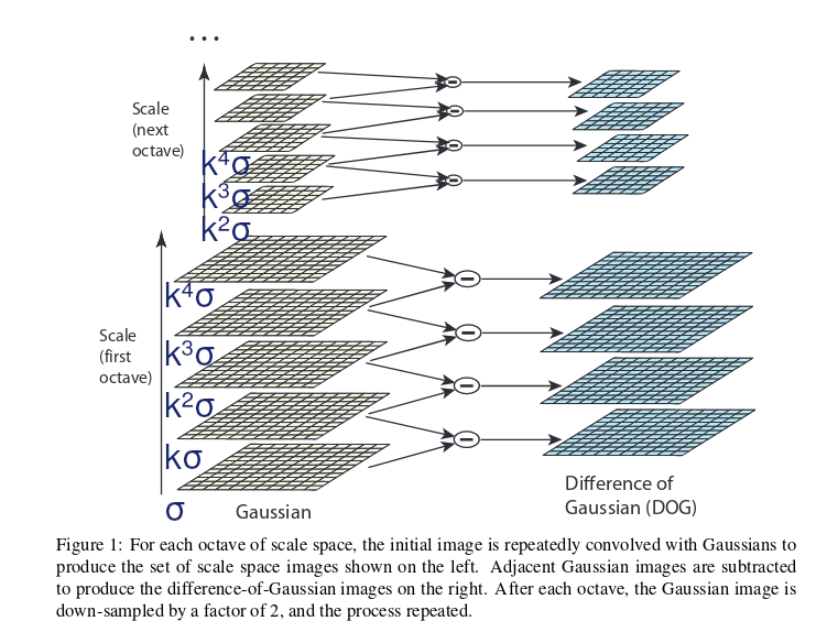
1. Uses DoG (Difference of Gaussian) to approximate Scale-normalized LoG (Laplacian of Gaussian)^[4].

   $$ G(x,y,\sigma) = \frac{1}{2 \pi \sigma^2} \exp^{- \frac{x^2 + y^2}{2 \sigma^2}} \\ D(x,y,\sigma) = (G(x,y,k \sigma) - G(x,y,\sigma)) * I(x,y) \\ G(x,y,k \sigma) - G(x,y,\sigma) \approx (k-1) \sigma^2 \nabla^2 G $$

   where \( G(x,y,\sigma) \) is the two dimensions Gaussian function, and \( I(x,y) \) is the input image.

2. [need more consideration] After each octave, the Gaussian image is down-sampled by a factor of 2, by resampling the Gaussian image that has twice the initial value of \( \sigma \) by taking every second pixel in each row and column. And we start on the new octave with \( k^2 \sigma \).

   

   Since the image size is reduced to 1/4, the sigma for the next octave becomes \( 2 k^4 \sigma \), which is equal to \( k^2 \sigma \).

   To understand it, frist consider this question: If the image size is reduced to 1\4, but the kernel size of the gaussian function remains the same, in order to produce the same effect as before, what should the new \( \sigma \) be?

   Given \( D_1 \) as an area in the original image, \( D_2 \) as the corresponding area in the new image, \( r_1 \) and \( r_2 \) are the radius of \( D_1 \) and \( D_2 \) respectively, then we have:

   $$ Area\_of(D_2) = \frac{1}{4} Area\_of(D_1) \\ r_2 = \frac{1}{2} r_1 $$

   Let the new \( \sigma \) be \( a \) times the original one, the question is now to solve the a for:

   $$ \iint_{D_1} G(x,y,\sigma) ,dx,dy = \iint_{D_2} G(x,y,a\sigma) ,dx,dy $$

   With the help of Gaussian Integral^[5], we can solve \( a \):

   $$ \begin{align*} \Rightarrow & 2 \pi \frac{1}{2 \pi \sigma^2} \int^{r_1}_{0} \exp^{- \frac{r^2}{2 \sigma^2}} r ,dr = 2 \pi \frac{1}{2 \pi a^2 \sigma^2} \int^{r_2}_{0} \exp^{- \frac{r^2}{2 a^2 \sigma^2}} r ,dr \\ \Rightarrow & - \sigma^2 (\exp^{- \frac{r_1^2}{2 \sigma^2}} - \exp^0) = \frac{1}{a^2} (- a^2 \sigma^2) (\exp^{- \frac{r_2^2}{2 a^2 \sigma^2}} - \exp^0) \\ \Rightarrow & a^2 = \frac{r_2^2}{r_1^2} \\ \Rightarrow & a = \frac{1}{2} \end{align*} $$

Puzzles

1. How the 3D interpolation (using Taylor expansion) works.

TODO

1. Continue at section 4.1 Eliminating edge responses.

References

David G. Lowe. 2004. Distinctive Image Features from Scale-Invariant Keypoints. Int. J. Comput. Vision 60, 2 (November 2004), 91-110. DOI: https://doi.org/10.1023/B:VISI.0000029664.99615.94
SIFT(Scale-Invariant Feature Transform) - Towards Data Science