Image Processing - Noise and denoise

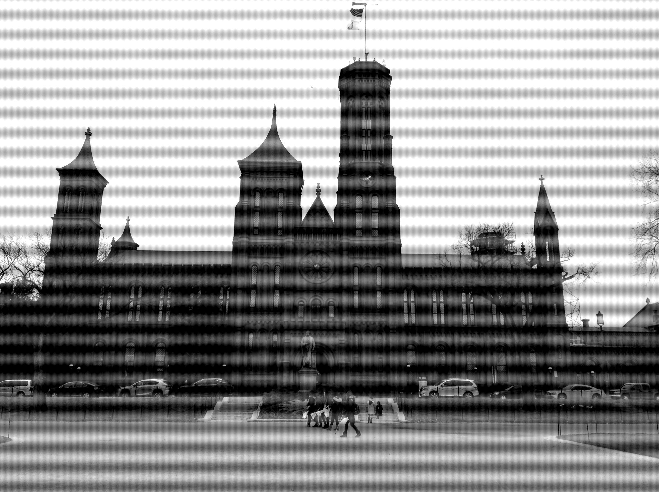
Types of Noise

Additive noise

Additive noise is independent from image signal. The image g with nosie can be considered as the sum of ideal image f and noise n.^[1]

$$ g = f + n $$

Multiplicative noise

Multifplicative noise is often dependent on image signal. The relation of image and noise is^[1]:

$$ g = f + fn $$

Gaussian noise

Gaussian noise, named after Carl Friedrich Gauss, is statistical noise having a probability density function (PDF) equal to that of the normal distribution, aka. the Gaussian distribution. i.e. the values that the noise can take on are Gaussian-distributed.

The PDF \( p \) of a Gaussian random variable \( z \) is given by^[2]:

$$ p_G(z) = \frac{1}{ \sigma \sqrt{2\pi} } e^{ - \frac{ (z-\mu)^2 }{ 2 \sigma^2 } } $$

Salt-and-pepper noise

Fat-tail distributed or "impulsive" noise is sometimes called salt-and-pepper nosie or spike noise. An image containing salt-and-pepper noise will have dark pixels in bright regions and bright pixels in dark regions.^[2]

The PDF of (Bipolar) Impulse noise is given by:

$$ p(z) = \left\{ \begin{array}{ll} p_a \qquad & for \, z = a \\ p_b \qquad & for \, z = b \\ 0 \qquad & otherwise \\ \end{array} \right. $$

if b > a, gray-level b appears as a light dot in the image. Conversely, level a appears like a dark dot. If either \( p_a \) or \( p_b \) is zero, the impulse noise is called unipolar.^[3]

Types of Filters^[4]

0. Spatial domain

1. Frequency domain (Transform domain)

2. Integrated Spatial and Frequency Domain

Spatial domain filtering

Low-pass filter

Typical low-pass filters can be:

$$ \frac{1}{9} \begin{bmatrix} 1 & 1 & 1 \\ 1 & 1 & 1 \\ 1 & 1 & 1 \\ \end{bmatrix} $$

and:

$$ \frac{1}{8} \begin{bmatrix} 0 & 1 & 0 \\ 1 & 4 & 1 \\ 0 & 1 & 0 \\ \end{bmatrix} $$

and a typical Gaussian filter:

$$ \frac{1}{16} \begin{bmatrix} 1 & 2 & 1 \\ 2 & 4 & 2 \\ 1 & 2 & 1 \\ \end{bmatrix} $$

More generally, a 2 dimensional Gaussian filter in spatial domain is:

$$ G(x,y) = \frac{1}{2 \pi \sigma^2} e^{- \frac{x^2+y^2}{2 \sigma^2}} $$

High-pass filter

Basically, we can obtain a high-pass filtering kernel corresponding to each of the low-pass filter kernels by subtracting the low-pass kernel from the all-pass kernel.^[5]

A typical high-pass filter can be:

$$ \frac{1}{9} \begin{bmatrix} -1 & -1 & -1 \\ -1 & 8 & -1 \\ -1 & -1 & -1 \\ \end{bmatrix} $$

and a typical Laplacian filter:

$$ \begin{bmatrix} 0.17 & 0.67 & 0.17 \\ 0.67 & -3.33 & 0.67 \\ 0.17 & 0.67 & 0.17 \\ \end{bmatrix} $$

Median filter

Replace a value with the median value of its surroundings.

$$ \begin{bmatrix} 2 & 4 & 1 \\ 3 & 8 & 1 \\ 2 & 5 & 1 \end{bmatrix} \Rightarrow \begin{bmatrix} 2 & 4 & 1 \\ 3 & 2 & 1 \\ 2 & 5 & 1 \end{bmatrix} $$

Frequency domain filtering

Low-pass filter

The Gaussian filter in frequency domain:

The derivation:

https://www.youtube.com/watch?v=iLQ-E0FA85Q

References

Shahriar Kaisar, et al. Salt and Pepper Noise Detection and removal by Tolerance based Selective Arithmetic Mean Filtering Technique for image restoration. (June 2008) International Journal of Computer Science and Network Security. Vol 8 No.6.
Tram Tran Nguyen Quynh, Hung Do Phi. Comparative Study of Image Denoise Algorithms