Decision Tree

Information Content

$$ I(X) = log_b(\frac{1}{P(X)}) $$

where,

• I : the information content of X. An X with greater I value contains more information.

• P : the probability mass function.

• \( log_b \) : b is the base of the logarithm used. Common values of b are 2 (bits), Euler's number e (nats), and 10 (bans).

Entropy (Information Theory)^[1]

$$ H(X) = E[I(X)] = E[-log(P(X))] $$

where,

• H : the entropy H. Named after Boltzmann's H-theorem (but the definition is proposed by Shannon). H indicates the uncertainty of X.

• P : probability mass function.

• I : the information content of X.

• E : the expected value operator.

The entropy can explicitly be written as:

$$ H(X) = - \sum_{i=1}^{n}{ P(x_i) log_b{P(x_i)} } $$

ID3^[2]

Use ID3 to build a decision tree:

0. Calculate the entropy \( E_0 \) of the samples under the current node.

1. Find a feature F that can maximize the information gain. The information gain is calculatd by:

   $$ \Delta{E} = E - E_0 $$

   where E is the entropy of the samples after being seperated by the feature F with the value V.

2. Use the feature F to seperate samples.

3. Repeat step 1 and 2 until the classification result is satisfactory.

Except from Shannon's Entropy, other measures can also be used to measure the impurity of the samples, such as Gini Impurity (aka. Square Impurity).

Gini Impurity:

$$ \begin{align*} I(N) &= \sum_{m \neq n}{ P(\omega_m) P(\omega_n) } \\ &= 1 - \sum_{j=1}^{k}{ P^2(\omega_j) } \end{align*} $$

ID4.5^[2]

In ID4.5, Information Gain Ratio is used instead of Information Gain.

$$ \Delta{E_R(N)} = \frac{ \Delta{E(N)} }{E(N)} $$

Continuous Values

ID4.5 supports features with continuous values by dividing the samples into two group with every possible value from the samples. Then chooses the division that maximize the Information Gain Ratio, and compares it with the other features' Information Gain Ratio.

Missing Values

Given all samples (in this node) as set \( D \), samples with property \( a \) (in this node) as set \( \tilde{D} \).

If the weight of each sample \( x \) is \( \omega_x \) (the initial weight is 1), we define:

$$ \begin{align*} \rho &= \frac{ \sum_{ x \in \tilde{D} }{ \omega_x } }{ \sum_{ x \in D }{ \omega_x } } \\ \tilde{p}_k &= \frac{ \sum_{ x \in \tilde{D}_k }{ \omega_x } }{ \sum_{ x \in \tilde{D} }{ \omega_x } } \quad ( 1 <= k <= |\gamma| ) \\ \tilde{r}_v &= \frac{ \sum_{ x \in \tilde{D}^v }{ \omega_x } }{ \sum_{ x \in \tilde{D} }{ \omega_x } } \quad ( 1 <= v <= V ) \end{align*} $$

where,

• \( \rho \) : the ratio of the weight of samples in \( \tilde{D} \) against the weight of all samples (in this node).

• \( \tilde{p}_k \) : the ratio of the weight of samples in \( \tilde{D} \) that belongs to class k against the weight of samples in \( \tilde{D} \).

• \( \tilde{r}_v \) : the ratio of the weight of samples that has value \( a^v \) for property \( a \) against the weight of samples in \( \tilde{D} \).

Then, we can calculate the information gain by:

$$ \begin{align*} Gain(D, a) &= \rho \times Gain(\tilde{D}, a) \\ &= \rho \times ( E(\tilde{D}) - \sum_{v=1}^{V}{ \tilde{r}_v E(\tilde{D}^v) } ) \end{align*} $$

And the entropy is calculated by:

$$ E(\tilde{D}) = - \sum_{k=1}^{|\gamma|}{ \tilde{p}_k log_2{\tilde{p}_k} } $$

Cutting Decision Trees (CDT)^[2]

We can cut a decision tree after it is built, or while it is being built.

Cutting a decision tree under construction means that if adding a child to a node will result in reducing in accuracy on validation set, no child will be added, and the node will turn into a leaf.

Cutting a decision tree after it is constructed:

0. First generate a decision tree from the training set.

1. Check each node, remove it if the accuracy on the validation set will improve without it.

CART (Classification And Regression Tree)

CART in regression:

Given a set of samples \( X \), and corresponding ground true outputs \( y \).

0. For a feature \( F \), choose a value \( V_m \), which divides the samples into two groups (one lager than value \( V_m \), one smaller or equal to value \( V_m \)). The output for group \( G_j \) is set to \( f_j \).

1. Choose the feature \( F \) and the value \( V_m \) and the outputs \( f_j \) that minimizes the square loss:

   $$ \begin{align*} & F, V_m, f_j = argmin_{F, V_m, f_j}( L(X) ) \\ & where, \\ & L(X) = \sum_{i=0}{N}{ (y_i - f(x_i))^2 } \\ & N = |X| (the number of samples in X) \\ & f(x_i) = f_j (x_i \in G_j) \\ \end{align*} $$

   It's obvious that \( f_j \) should be the average of the outputs for samples in group \( G_j \):

   $$ f_j = ave(y_i | x_i \in G_j) $$

   So we just need to loop through features and possible values to find \( F \) and \( V_m \).

The algorithm:

import numpy as np

def CART_next_node(X, Y):
    samples_count, features_count = np.shape(X)
    
    best_F = np.nan; best_V = np.nan; min_L = np.inf
    for F in range(0, features_count):
        XF = X[:, F]

        min_V = np.nan; min_Lv = np.inf
        for V in XF:
            if (XF <= V).all(): continue
            f1 = np.average(Y[XF <= V])
            f2 = np.average(Y[XF > V])
            Lv = np.sum([
                np.square( y - (lambda x: (f1 if x <= V else f2))(x) )
                for x, y in zip(XF, Y)
            ])
            if Lv < min_Lv:
                min_V = V
                min_Lv = Lv

        if min_Lv < min_L:
            best_F = F
            best_V = min_V
            min_L = min_Lv

    return best_F, best_V, min_L

A test result:

This (CART) yields piecewise constant models. Although they are simple to interpret, the prediction accuracy of these models often lags behind that of models with more smoothness.

It can be computationally impracticable, however, to extends this approach to piecewise linear models, because two linear models (one for each child node) must be fitted for every candidate split.

(So there is M5', an adaptation of a regression tree algorithm by Quinlan, which uses a more computationally efficient strategy to construct piecewise linear models.)

— Wei-Yin Loh.
(2011). Classification and regression trees.^[3]

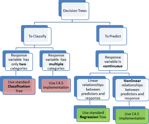
The map^[4]

Reference