Classification And Overfitting

This is a learning note of Logistic Regression of Machine Learning by Andrew Ng on Coursera.

Hypothesis Representation

Uses the "Sigmoid Function," also called the "Logistic Function":
$$ h_{\theta}(X) = g( \theta^{T} X ) \\ z = \theta^{T} X \\ g(z) = \frac{1}{ 1 + e^{-z} } \\ $$ Which turn linear regression into classification.

Sigmoid function looks like this:
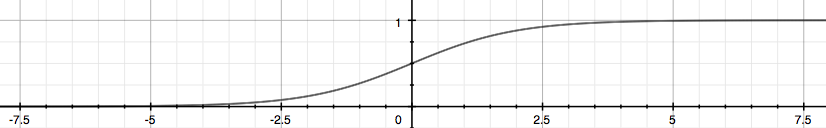\( h_{\theta}(x) \) give us the probability that the output is 1.
$$ h_{\theta}(x) = P(y = 1 | x; \theta) = 1 - P(y = 0 | x; \theta) $$

In fact, \( z = \theta^{T} X \) is simplified as
$$ z = \theta_0 + \theta_1 x_1 + \theta_2 x_2 + \dots $$ for logistic regression, and is
$$ z = \theta_0 + \theta_1 x + \theta_2 x^2 + \dots $$ for linear regression. In some complicated case, z might be something like:
$$ z = \theta_0 + \theta_1 x_1 + \theta_2 x_1^2 + \theta_3 x_2 + \theta_4 x_1 x_2 + \dots $$

Decision Boundary

Decision boundary is the line (or hyperplane) that separates the area where y = 0 and where y = 1 (or separates different classes). It's created by our hypothesis function.

The input to the sigmoid function is not necessary to be linear, and could be a function that describes a circle (e.g. \( z = \theta_0 + \theta_1 x_1^2 + \theta_2 x_2^2 \)) or any shape to fit the data.

Cost Function

Using the cost function for linear regression in classification will cause the output to be wavy, resulting in many local optima. i.e. it is not a convex function.
The cost function for logistic regression looks like:
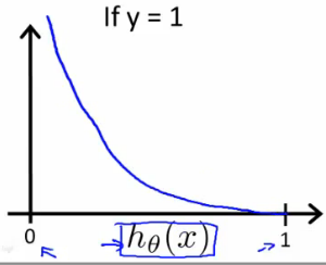
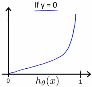
$$ J(\theta) = \frac{1}{m} \sum_{i=1}^{m} Cost( h_\theta(x^{(i)}), y^{(i)} ) \\ Cost( h_\theta(x), y ) = \begin{cases} -log( h_\theta(x) ) & \text{if y = 1} \\ -log( 1 - h_\theta(x) ) & \text{if y = 0} \\ \end{cases} $$ \( (x^{(i)}, y^{(i)}) \) refers to the \( i^{th} \) training example.

When y = 1, plot for \( J(\theta) \) vs \( h_\theta(x) \) :
When y = 0, plot for \( J(\theta) \) vs \( h_\theta(x) \) :

Compress the two conditional cases into ones, we get a simplified cost function:
$$ Cost( h_\theta(x), y) = -y log( h_\theta(x) ) - (1 - y) log( 1 - h_\theta(x) ) \\ J(\theta) = - \frac{1}{m} \sum_{i=1}^{m} \left[ y^{(i)} log( h_\theta( x^{(i)} ) ) + (1 - y^{(i)}) log( 1 - h_\theta( x^{(i)} ) ) \right] $$ Vectorized:
$$ h = g(X\theta) \\ J(\theta) = \frac{1}{m} \cdot ( -y^T log(h) - (1 - y)^T log(1 - h) ) $$

Gradient Descent

Generally, gradient descent is in this form:
$$ \begin{align*} & Repeat \; \{ \\ & \qquad \theta_j := \theta_j - \alpha \frac{\partial}{\partial \theta_j} J(\theta) \\ & \} \end{align*} $$

Work out the derivative part using calculus:
$$ \begin{align*} & Repeat \: \{ \\ & \qquad \theta_j := \theta_j - \frac{\alpha}{m} \sum_{i=1}^{m} (h_\theta( x^{(i)} ) - y^{(i)}) x_j^{(i)} \\ & \} \end{align*} $$

Vectorized:
$$ \theta := \theta - \frac{\alpha}{m} X^T (g(X\theta) - \vec{y}) \\ ( \text{where} \: X = \begin{bmatrix} x_{0}^{(1)} & x_{1}^{(1)} & x_{2}^{(1)} & \dots & x_{n}^{(1)} \\ x_{0}^{(2)} & x_{1}^{(2)} & x_{2}^{(2)} & \dots & x_{n}^{(2)} \\ \vdots & \vdots & \vdots & \ddots & \vdots \\ x_{0}^{(m)} & x_{1}^{(m)} & x_{2}^{(m)} & \dots & x_{n}^{(m)} \\ \end{bmatrix} , \: \theta = \begin{bmatrix} \theta_{0} \\ \theta_{1} \\ \vdots \\ \theta_{n} \\ \end{bmatrix} ) $$

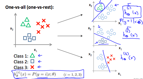
Multiclass Classification: One-vs-all

In Multiclass classification, y = {0, 1, ..., n} instead of y = {0, 1}. But we can still use the similar strategy as what we use for two-class classification. We can regard one class as 1 and the others as 0, and train a logistic regression classifer \( h_\theta(x) \) for it. And repeat this process for other classes. At the end, we choose the one with the max possiblity to be the predicted class.
$$ y \in {0, 1, ..., n} \\ h_\theta^{(0)}(x) = P(y = 0 | x; \theta) \\ h_\theta^{(1)}(x) = P(y = 1 | x; \theta) \\ \dots \\ h_\theta^{(n)}(x) = P(y = n | x; \theta) \\ prediction = \max_i( h_\theta^{(i)}(x) ) $$ This image shows how one could classify 3 classes:

Solve the Problem of Overfitting

If we try to add too much features, e.g. \( y = \sum_{j=0}{5} \theta_j x^j \) for the example below, we will get a wiggly and curvy curve which fit the traning data perfectly - but not the testing data. That's what the problem of overfitting.

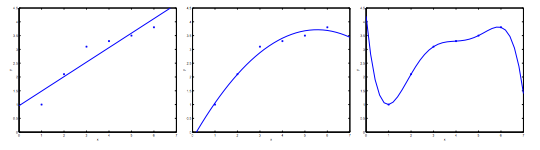
Underfitting, or high bias, is when the hypothesis function maps poorly to the trend of the data. On the contrary, overfitting, or high variance, is caused by a hypothesis function which fits the avaliable data but does not generalize well to predict new data.

To address the issue of overfitting, one can:

1. Reduce the number of features;
   • Manually select features to keep.
   • Use a model selection algorithm.
2. Regularization;
   • Keep all features, but reduce the magnitude of parameter \( \theta_j \).
   • Regularization works well when we have a lot of slighty useful features.

Regularization

Add a regularization parameter \( \lambda \) to \( \theta \) to penalize those slighty useful features. But be careful - if lambda is too large, it may smooth out the function too much and cause underfitting.
$$ J(\theta) = \frac{1}{m} \sum_{i=1}^{m} Cost(h_\theta( x^{(i)} ), y^{(i)}) + \lambda \sum_{j=1}^{m} \theta_j \\ $$

Gradient Descent (Notice that we don't need to penalize \( \theta_0 \).):
$$ \begin{align*} & Repeat \: \{ \\ & \qquad \theta_j := \theta_j - \alpha \frac{\partial J(\theta)}{\partial \theta_j} \hspace{5em} j \in [ {0, 1, ..., n} ] \\ & \} \end{align*} $$

Regularized Linear Regression

For regularized linear regression:
$$ J(\theta) = \frac{1}{2m} \sum_{i=1}^{m} (h_\theta(x^{(i)}) - y^{(i)})^2 $$ Normal Equation:
$$ \theta = (X^T X + \lambda \cdot L )^{-1} X^T y \\ ( \text{where} \: L = \begin{bmatrix} 0 & \\ & 1 & \\ & & 1 & \\ & & & \ddots & \\ & & & & 1 & \\ \end{bmatrix} ) $$ If m < n, then \( X^T X \) is non-invertible. However, when we add the term \( \lambda \cdot L \) , then \( X^T X + \lambda \cdot L \) becomes invertible.

A proof for normal equation (Ref: Derivation of the normal equation for linear regression):
$$ \begin{align*} \qquad & J(\theta) = \frac{1}{2m} (X\theta - y)^T (X\theta - y) \\ \Rightarrow & 2m \cdot J(\theta) = ((X\theta)^T - y^T)(X\theta - y) \\ \Rightarrow & 2m \cdot J(\theta) = (X\theta)^T X\theta - (X\theta)^T y - y^T (X\theta) + y^T y \\ & \text{(Notice that } (X\theta)^T y = y^T (X\theta) \text{. So we have:)} \\ \Rightarrow & 2m \cdot J(\theta) = (X\theta)^T X\theta - 2 (X\theta)^T y + y^T y \\ \end{align*} $$ Now let:
$$ \frac{\partial J}{\partial \theta} = 2 X^T X \theta - 2 X^T y = 0 $$ We get:
$$ X^T X \theta = X^T y $$ That is:
$$ \theta = (X^T X)^{-1} X^T y $$

Regularized Logistic Regression

For regularized logistic regression:
$$ J(\theta) = - \frac{1}{m} \sum_{i=1}^{m} \left[ y^{(i)} log(h_\theta(x^{(i)})) + (1 - y^{(i)}) log(1 - h_\theta(x^{(i)})) \right] + \frac{\lambda}{2m} \sum_{j=1}^{n} \theta_j^2 $$

Gradient descent:
$$ \begin{align*} & Repeat \: \{ \\ & \qquad \theta_0 := \theta_0 - \frac{\alpha}{m} \sum_{i=1}^{m} (h_\theta( x^{(i)} ) - y^{(i)}) x_0^{(i)} \\ & \qquad \theta_j := \theta_j - \frac{\alpha}{m} \left[ \sum_{i=1}^{m} (h_\theta( x^{(i)} ) - y^{(i)}) x_j^{(i)} + \lambda \theta_j \right] \hspace{5em} j \in [ {1, 2, ..., n} ] \\ & \} \end{align*} $$