R-CNN

Overview

Regions with CNN features:

1. Efficient Graph Based Image Segmentation
   • use disjoint set to speed up merge operation
2. Selective Search
   • HOG (Histogram of Oriented Gradient)
   • Multiple criterions (color, texture, size, shape) to merge regions
3. AlexNet/VGG16
4. R-CNN

Notice that many descriptions are replicated from the orignal sources directly.

Some Fundermental Conceptions

Batch Size

1. Stochastic Gradient Descent. Batch Size = 1
2. Batch Gradient Descent. Batch Size = Size of Training Set
3. Mini-Batch Gradient Descent. 1 < Batch Size < Size of Training Set

Regularization

A regression model that uses L1 Regularization technique is called Lasso Regression and model which uses L2 is called Ridge Regression.

1. Ridge Regularization

   Ridge regression adds "squared magnitude" of coefficient as penalty term to the loss function.

   $$ \sum_{i=1}^{n} (y_i - \sum_{j=1}^{p} x_{ij} \beta_j)^2 + \lambda \sum_{j=1}^{p} \beta_j^2 $$

   The first sum is an example of loss function.

2. Lasso Regularization

   Lasso Regression (Least Absolute Shrinkage and Selection Operator) adds "absolute value of magnitude" of coefficient as penalty term to the loss function.

   $$ \sum_{i=1}^{n} (y_i - \sum_{j=1}^{p} x_{ij} \beta_j)^2 + \lambda \sum_{j=1}^{p} | \beta_j | $$

Backpropagation

Efficient Graph Based Image Segmentation^[1]

Efficient Graph Based Image Segmentation presents by Felzenszwalb and Huttenlocher.

Definitions

1. Expression \( Int(C) \) : The internal difference of component \( C \subseteq V \) , (V is the vertices set of the graph).

   $$ Int(C) = max_{e \in MST(C, E)} w(e) $$

   where,

   \( MST(C, E) \) : The minimum spanning tree of the component C in the graph with edges set E.

2. Expression \( MInt(C_1, C_2) \) : Minimum internal difference.

   $$ MInt(C_1, C_2) = min(Int(C_1) + \tau(C_1), Int(C_2) + \tau(C_2)) $$

   where,

   \( \tau \) is a threshold function which controls the degree to which the difference between two components must be greater than their internal differences in order for there to be evidence of a boundary between them.

   $$ \tau(C) = k / | C | $$

3. Expression \( Dif(C_1, C_2) \) : The difference between two components \( C_1, C_2 \subseteq V \) , defined as the minimum weight edge connecting the two componets.

   $$ Dif(C_1, C_2) = min_{v_i \in C_1, v_j \in C_2, (v_i, v_j) \in E} w((v_i, v_j)) $$

4. Expression \( D(C_1, C_2) \) : The region comparison predicate. If true, the two components are distinct and should NOT be merged. If false, the two components should be merged.

   $$ D(C_1, C_2) = \begin{cases} true, & \text{if} Dif(C_1, C_2) \gt MInt(C_1, C_2) \\ false, & \text{otherwise} \\ \end{cases} $$

Key Points

1. It's important for internal differences to be the max weight of the edge in MST, instead of all edges. Or the difference will might grow too large.

2. To speed up the merging process, Union-find Set (or Disjoint Set) can be applied to tag the components in the same segment.

Selective Search^[2][3]

The algorithm

Input: (colour) image
Output: Set of object location hypotheses L

Obtain initial regrions \( R = {r_1, ..., r_n} \) using Felzenszwalb and Huttenlocher (2004); 
Initialise similarity set \( S = \emptyset \) ;

foreach Neighbouring region pair \( (r_i, r_j) \) do

Calculate similarity \( s(r_i, r_j) \) ;
\( S = S \cup s(r_i, r_j) \) ;

while \( S \ne \emptyset \) do

Get highest similarity \( s(r_i, r_j) = max(S) \) ;
Merge corresponding regions \( r_t = r_i \cup r_j \) ;
Remove similarities regarding \( r_i: S = S \backslash s(r_i, r_*) \) ;
Remove similarities regarding \( r_j: S = S \backslash s(r_*, r_j) \) ;
Calculate similarity set \( S_t \) between \( r_t \) and its neighbours;
\( S = S \cup S_t \) ;
\( R = R \cup r_t \) ;

Extract object location boxes L from all regions in R;

Diversification Strategies

1. Expression \( S_{colour} \) for colour similarity

   $$ S_{colour} (r_i, r_j) = \sum_{k=1}^{n} min(c_i^k, c_j^k) $$

   where,

   \( c_i \) : the colour histogram of region \( r_i \) , and \( c_{r_i \cup r_j} = \frac{ size(r_i) \times c_i + size(r_j) \times c_j }{ size(r_i) + size(r_j) } \)

   One can use numpy.histogram for the calculation of colour histograms.

   Both colour histograms and texture histograms are normalised using the \( L_1 \) norm.

2. Expression \( S_{texture} \) for texture similarity

   $$ S_{texture} (r_i, r_j) = \sum_{k=1}^{n} min(t_i^k, t_j^k) $$

   where,

   \( t_i \) : the texture histogram of region \( r_i \)

   The texture histogram is a combination of histograms, which are extracted from eight orientations of Gaussian derivative using \( \theta = 1 \) for each colour channel. For each orientation for each colour channel, the histogram is extracted using a bin size of 10. This leads to a texture histogram \( t_i = { t_i^1, ..., t_i^n } \) for each region \( r_i \) with dimensionality n = 240 when three colour channels are used.

   Here is how to calculate Gaussian derivative in eight orientation for one colour channel:

   # By Donny (https://github.com/Donny-Hikari)
   
   import numpy as np
   import skimage as ski
   
   def calc_gradient_1channel(I, mode='ignore'):
       '''
       Oriented Gradient (directional derivative):
       \delta_v G = v \dot (Gy \times d Gx / dx + Gx \times d Gy / dy)
       But there is a more simple solution:
       \delta_v(G) * I \delta_v(I * G) = \delta_v(I) * G
       Thanks to hints from skimage.feature.hog
       Note that in the 'ignore' mode, all edges responses are 0
   
       Params
       ------
       I: pixels array of shape (height, width)
   
       mode: 'ignore' or 'reflect'
           'ignore': set all edges responses to 0
           'reflect': reflect outer values at edges
       '''
       height, width = np.shape(I)
       g_col = np.empty((height, width), dtype=np.float64)
       g_row = np.empty((height, width), dtype=np.float64)
   
       # an equivalent implement for the 'reflect' mode:
       # g_col = scipy.ndimage.convolve(I, [[1],[0],[-1]], mode='reflect)
       # g_row = scipy.ndimage.convolve(I, [[1,0,-1]], mode='reflect')
       if mode == 'ignore':
           g_col[0, :] = 0
           g_col[-1, :] = 0
           g_row[:, 0] = 0
           g_row[:, -1] = 0
       elif mode == 'reflect':
           g_col[0, :] = I[1, :] - I[0, :]
           g_col[-1, :] = I[-1, :] - I[-2, :]
           g_row[:, 0] = I[:, 1] - I[:, 0]
           g_row[:, -1] = I[:, -1] - I[:, -2]
       
       g_col[1:-1, :] = I[2:, :] - I[:-2, :]
       g_row[:, 1:-1] = I[:, 2:] - I[:, :-2]
       
       return g_col, g_row
   
   def calc_gdfd_1channel(I, orientations=8):
       '''
       gaussian directional first derivative
       '''
       g_col, g_row = calc_gradient_1channel(I)
       g_col = ski.filters.gaussian(g_col, sigma=1)
       g_row = ski.filters.gaussian(g_row, sigma=1)
       gdfd_Is = [None] * orientations
       for o in range(orientations):
           theta = o * np.pi / orientations # theta = o * sympy.pi / orientations
   
           # the following three lines
           v = np.array([np.sin(theta), np.cos(theta)]) # Note that np.cos(np.pi/2) != np.sin(0.0)
           ogI = (v.reshape((2,1,1)) * [g_col, g_row]).sum(axis=0)
           gdfd_Is[o] = ogI
           # is equal to the following line
           # gdfd_Is[o] = np.sin(theta) * g_col + np.cos(theta) * g_row
   
           # Performing gaussian on g_col and g_row before the calculation,
           # is equals to performing gaussian on the final result.
           # gdfd_Is[o] = ski.filters.gaussian(gdfd_Is[o], sigma=1)
   
           # Note that the result (gdfd_Is[o]) may be slightly over the range (0.0, 1.0)
           # assert(gdfd_Is[o].dtype == np.float64)
           # assert((gdfd_Is[o] >= -1.0).all() and (gdfd_Is[o] <= 1.0).all())
       return gdfd_Is
   
   
   
   
   

3. Expression \( s_{size} \) for size similarity

   $$ s_{size} (r_i, r_j) = 1 - \frac{ size(r_i) + size(r_j) }{ size(im) } $$

   where,

   \( size(im) \) : the size of the image in pixels

   \( s_{size} \) encourages small regions to merge early.

4. Expression \( s_{fill} \) for fill similarity

   $$ s_{fill} (r_i, r_j) = 1 - \frac{ size(B B_{ij}) - size(r_i) - size(r_j) } { size(im) } $$

   where

   \( B B_{ij} \) : the tight bounding box around \( r_i \) and \( r_j \)

   \( s_{fill} \) measures how well regions fit with each other. If region \( r_i \) is close to or is contained in region \( r_j \) , it is logical to merge them first to avoid holes.

5. Expression Combine all four strategies

   $$ s(r_i, r_j) = a_1 s_{colour} (r_i, r_j) + a_2 s_{texture} (r_i, r_j) + a_3 s_{size} (r_i, r_j) + a_4 s_{fill} (r_i, r_j) $$

   where

   \( a_i \) : denotes if the similarity measure is used or not, \( a_i \in \{0, 1\} \)

AlexNet^[4]

Reducing Overfitting - Data Augmentation

Krizhevsky, et. al. ^[4] employed two distinct forms of data augmentation.

1. Generating image translations and horizontal reflections.

   At training time: Extract random \( 224 \times 224 \) patches (and their horizontal reflections) from the \( 256 \times 256 \) images.

   At test time: Extract five \( 224 \times 224 \) patches (the four corner patches and the center patch) as well as their horizontal reflections (hence ten patches in all), and average the predictions made by the network's softmax layer on the ten patches.

2. Altering the intensities of the RGB channels in training images.

   The object identity is invariant to changes in the intensity and color of the illumination, therefore this scheme is used to approximately capture this important property of natural images.

   First of all, perform PCA on the set of RGB pixel values throughout the ImageNet training set.

   # By Donny (https://github.com/Donny-Hikari)
   
   import numpy as np
   
   def calc_covariances(bs=None):
       print(TERMCONST.CLL, end='')
       print('loading training dataset')
       train_X, train_y = load_data('train', verbose=True)
       print(TERMCONST.CLL, end='')
   
       n_sample, n_imgh, n_imgw, n_channels = train_X.shape
       n_observations = n_sample * n_imgh * n_imgw
   
       print('reshaping')
   
       if bs == None:
           train_X = train_X.reshape((n_observations, n_channels))
       else:
           tmp_X = []
           for ind in range(0, n_sample, bs):
               tmp_X.append(train_X[:bs].reshape(len(train_X[:bs]) * n_imgh * n_imgw, n_channels))
               train_X = train_X[bs:]
           train_X = np.concatenate(tmp_X)
   
       chunk_size = 1024 * 1024
   
       print('calculating means')
   
       means = np.zeros(n_channels, dtype=np.float)
       for ind in range(0, n_observations, chunk_size):
           means += train_X[ind:ind+chunk_size].sum(axis=0) / n_observations
       print(means)
   
       # slow
       # print(train_X.mean(axis=0, dtype=np.float))
   
       print('calculating covariances')
   
       covariances = np.zeros((n_channels, n_channels), dtype=np.float)
       for row in range(n_channels):
           for col in range(n_channels):
               for ind in range(0, n_observations, chunk_size):
                   covariances[row][col] += np.sum((train_X[ind:ind+chunk_size, row]-means[row])/255 * (train_X[ind:ind+chunk_size, col]-means[col])/255) / (n_observations-1)
       print(covariances)
   
       # memory error
       # print(np.cov(train_X, rowvar=False))
   
       eigenvalues, eigenvectors = np.linalg.eig(corvariances)
       return eigenvalues, eigenvectors
   
   
   
   
   
   

   Then, to each training image, add multiples of the found principal components, with magnitudes proportional to the corresponding eigenvalues times a random variable drawn from a Gaussian with mean 0 and standard deviation 0.1.

   $$ [RI^R, RI^G, RI^B] = [I^R, I^G, I^B] + [p_1, p_2, p_3] [\alpha_1 \lambda_1, \alpha_2 \lambda_2, \alpha_3 \lambda_3]^T $$

   where,

   RI: the output image for training

   I: the input image

   p: the eigenvectors of the \( 3 \times 3 \) covariance matrix of RGB pixel values

   \( \lambda \) : the eigenvalues of the \( 3 \times 3 \) covariance matrix of RGB pixel values

   \( \alpha \) : the random factor, drawn only once for all the pixels of I each time I presents

Reducting Overfitting - Dropout

Dropout is also a common way to tackle overfitting. Refers to the original paper^[4] for more details about dropout.

Initializing Neuron Weights

The weights in each layer is initialized from a zero-mean Gaussian distribution with standard de-viation 0.01. The neuron biases in the second, fourth, and fifth convolutional layers, as well as in the fully-connected hidden layers, is initialized with the constant 1. This initialization accelerates the early stages of learning by providing the ReLUs with positive inputs. The neuron biases in the remaining layers is initialized with the constant 0.

VGG^[5]

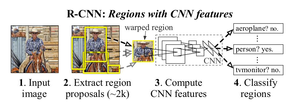
R-CNN^[6]

Object detection system overview:

1. Supervised pre-training

   Discriminatively pre-train the CNN on a large auxiliary dataset (ILSVRC2012 classification) using image-level annotations only.

   This step is important for discriminating the background from the objects in the latter step. Notice that it should be carried out on a large auxiliary dataset. When I tried to reproduce R-CNN, I pre-trained the AlexNet on the same dataset (VOC2012) that I used in the latter step. And the final mAP is only around 10%. After changing to the pre-trained VGG in keras, the final mAP is immediately improved to 38%.

2. Domain-specific fine-tunning

   To adapt the CNN to the detection task and the new domain (warped proposal windows), training is countinue with stochastic gradient descent (SGD) using only warped region proposals.

3. Object category classifiers - compressing features using SVM

   No implemented yet

4. Object proposal transformations

   Multiple tricks apply in object proposal transformations.

   1. To warp or to scale isotropically.

      R. Girshick et. al. compared these two methods. The isotropic scaling method encloses each object proposal inside the tightest square and then scales it to the CNN input size. The warp method anisotropically scales each object proposal to the CNN input size.

      The isotropic scaling method keeps the ratio information, at the cost of creating blank area (filled with the image mean) in the input image which provides few information.

      The anisotropic scaling (warp) method loses the ratio information, while maximizing the use of space.

   2. To add additional image context or not.

      It is found by experiments that adding context padding improves mAP significantly. The best context padding found by limited experiments is 16 pixels.

5. Bounding-box regression

   No implemented yet

TODOs

1. Loss function for CNN
2. SIFT
3. Batch size
4. Backpropagation
5. Optimizer

References