Mathematical Basis - Squashing Function
This article is about some squashing functions of deep learning, including Softmax Function, Sigmoid Function, and Hyperbolic Functions. All of these three functions are used to squash value to a certain range.
Softmax Function
Softmax Function: A generalization of the logistic function that "squashes" a K-dimensional vector z of arbitrary real values to a K-dimensional vector $$ \sigma ( \mathbf z ) $$ of real values, where each entry is in the range (0, 1], and all the entries add up to 1.
$$ {\displaystyle \sigma : \mathbb{R}^{K}\to \left{ \sigma \in \mathbb{R}^{K} | \sigma_{i} > 0, \sum_{i=1}^{K} \sigma_{i} = 1 \right}} $$
$$ \sigma ( \mathbf{z} )_{j}={ \frac{e^{z_{j}}}{ \sum_{k=1}^{K} e^{z_{k}} } } \quad \text{for j=1, ..., K.} $$
In probability theory, the output of the softmax function can be used to represent a categorical distribution - that is, a probability distribution over K different possible outcomes.
The softmax function is the gradient of the LogSumExp function.
LogSumExp Function
LogSumExp Function: The LogSumExp(LSE) function is a smooth approximation to the maximum function.
$$ LSE(x_1, ..., x_n) = log(\sum_{i=1}^{n} e^{x_i}) $$
($$log$$ stands for the natural logarithm function, i.e. the logarithm to the base e.)
When directly encountered, LSE can be well-approximated by $$ max { x_1, ..., x_n } $$ :
$$ max { x_1, ..., x_n } \leq LSE(x_1, ..., x_n) \leq max { x_1, ..., x_n } + log(n) $$
Sigmoid Function
Sigmoid Function: A mathematical function with a "S"-shaped curve.
One frequent used sigmoid function in ML is the logistic function.
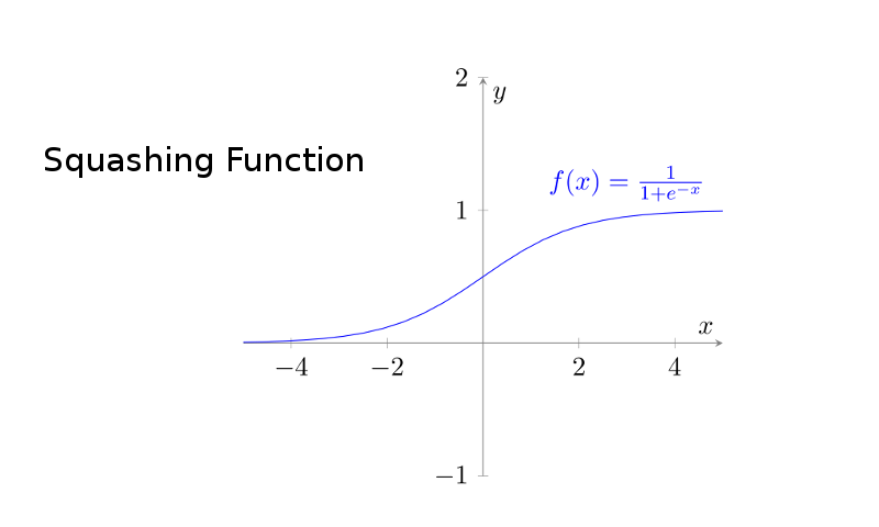
Logistic Function:
$$ f(x) = \frac{1}{1+e^{-x}} $$
$$ \tikz \node [scale=1.1] { \begin{tikzpicture}[] \begin{axis}[ axis line style=gray, ymin=-1, ymax=2, axis x line=center, axis y line=center, xlabel=$x$, ylabel=$y$ ] \addplot[blue]{1/(1+exp(-x))}; \addplot[blue] coordinates{(3,1.2)} node{$f(x)=\frac{1}{1+e^{-x}}$}; \end{axis} \end{tikzpicture} }; $$
To understand how it work, first we differentiate it:
$$ f\prime(x) = \frac{1}{2+e^{x}+e^{-x}} $$
$$ \tikz \node [scale=1.1] { \begin{tikzpicture}[] \begin{axis}[ axis line style=gray, ymin=-1, ymax=1, axis x line=center, axis y line=center, xlabel=$x$, ylabel=$y$ ] \addplot[blue]{1/(2+exp(x)+exp(-x))}; \addplot[blue] coordinates{(3,0.3)} node{$f(x)=\frac{1}{2+e^{x}+e^{-x}}$}; \end{axis} \end{tikzpicture} }; $$
Since function $$ g(x) = e^{x}+e^{-x} $$ is a (hyperbolic ?) curve which looks like a quadratic function, it's clear that $$ f\prime(x) $$ will go up to 0.25 from 0, from negative infinity to 0, and than go down to 0 again, from 0 to positive infinity.
So from the derivative, we can see that logistic function will be in "S"-shape, with its value very close to 0 when x getting closer and closer to negative infinity, and with its value very close to 1 when x getting near positive infinity. The turning point of tendency is 0, where the second derivative is 0 and where the value of the logistic function is 0.5.
Hyperbolic Function
Inspired by Euler's formula, $$ e^{i\theta} = cos(\theta) + i sin(\theta) $$, hyperbolic functions extend the notion of the parametric equations for a unit circle to the parametric equations for a hyperbola. ( From Hyperbolic Trigonometric Function | Brilliant Math & Science Wiki )
Notice: Hyperbolic Tangent is also a sigmoid function according to wikipedia Sigmoid Function.
Six hyperbolic functions :
| hyperbolic | connection with trigonometric | |
|---|---|---|
| sine | $$ sinh(x) = \frac{e^x - e^{-x}}{2} $$ | $$ sinh(x)=-i sin(ix) $$ |
| cosine | $$ cosh(x) = \frac{e^x + e^{-x}}{2} $$ | $$ cosh(x) = cos(ix) $$ |
| tangent | $$ tanh(x) = \frac{e^x - e^{-x}}{e^x + e^{-x}} = \frac{1-e^{-2x}}{1+e^{-2x}} $$ | $$ tanh(x) = -i tan(ix) $$ |
| cotangent ($$ = \frac{1}{tan(x)} $$) | $$ coth(x) = \frac{e^x + e^{-x}}{e^x - e^{-x}} , \quad {x \ne 0} $$ | $$ coth(x) = i cot(ix) $$ |
| secant ($$ = \frac{1}{cos(x)} $$) | $$ sech(x) = \frac{2}{e^x + e^{-x}} $$ | $$ sech(x) = sec(ix) $$ |
| cosecant ($$ = \frac{1}{sin(x)} $$) | $$ csch(x) = \frac{2}{e^x - e^{-x}} , \quad {x \ne 0} $$ | $$ csc(x) = i csc(ix) $$ |
Graph of these functions :
$$ \tikz \node [scale=1.1] { \begin{tikzpicture}[] \begin{axis}[ samples=120, axis line style=gray, ymin=-5, ymax=5, axis equal, axis x line=center, axis y line=center, xlabel=$x$, ylabel=$y$, ] \addplot[green]{(exp(x)-exp(-x))/2}; \addlegendentry{sinh} \addplot[red]{(exp(x)+exp(-x))/2}; \addlegendentry{cosh} \addplot[blue]{(exp(x)-exp(-x))/(exp(x)+exp(-x))}; \addlegendentry{tanh} \end{axis} \end{tikzpicture} }; $$
$$ \tikz \node [scale=1.1] { \begin{tikzpicture}[] \begin{axis}[ samples=120, axis line style=gray, ymin=-5, ymax=5, axis equal, axis x line=center, axis y line=center, xlabel=$x$, ylabel=$y$, ] \addplot[green, restrict expr to domain={(x<-0.1)+(x>0.1)}{0.1:+inf}]{(exp(x)+exp(-x))/(exp(x)-exp(-x))}; \addlegendentry{coth} \addplot[red]{2/(exp(x)+exp(-x))}; \addlegendentry{sech} \addplot[blue, restrict expr to domain={(x<-0.1)+(x>0.1)}{0.1:+inf}]{2/(exp(x)-exp(-x))}; \addlegendentry{csch} \end{axis} \end{tikzpicture} }; $$
Original Link: https://blog.ny-do.com/posts/6879787930/